Chapter structure
- 11.1 Development, Modern Application and Interpretation of
Feynman Diagrams - 11.2 Feynman’s Struggle for a Physical Interpretation
of the Dirac Equation - 11.3 Zitterbewegung
- 11.4 Positrons and Interaction
- 11.5 Abandoning the Search for a Microscopic Analysis
- 11.6 Solution to the Problems through an Appropriate
Representation of the Phenomena - 11.7 Comparison to Other Developments of Concepts and Means
of Representation - Abbreviations and Archives
- Acknowledgements
- References
- Footnotes
Around the year 1948, Richard Phillips Feynman (1918–1988) began to use a particular kind of diagram for the theoretical treatment of recalcitrant problems in the theory of quantum electrodynamics (QED), that is, the calculation of the self-energy of the electron. Soon thereafter, these so-called Feynman diagrams became a ubiquitous tool in theoretical elementary particle physics.
In this contribution, I first briefly sketch how Feynman diagrams are used today, how they are most often interpreted and how their genesis is usually described, see sec. (11.1). In the second part I present my reconstruction of how Feynman, starting from a search for an appropriate interpretation of the “Dirac equation” (Dirac 1928), arrived at an innovative representation of quantum electrodynamic phenomena, see sects. (11.2)–(11.5).
My reconstruction of Feynman’s struggle is based on manuscript pages which the Archives of the California Institute of Technology (Caltech) kindly made accessible to me. Some of these manuscript pages can also be found in Silvan Schweber’s book on QED (Schweber 1994) and in some of his articles, for example (Schweber 1986). I hope, however, that my reconstruction of the material reveals more clearly how Feynman’s diagrammatic representations were the means by which he defined and further developed physical models to interpret theoretical equations.
The third and last part is concerned with Freeman Dyson’s systematization and theoretical updating of Feynman’s framework, see sec. (11.6).1 I end with a comparison with two other case studies concerning developments of concepts and means of representation, see sec. (11.7).
11.1 Development, Modern Application and Interpretation of
Feynman Diagrams
The modern application of Feynman diagrams goes something like this: To calculate, for instance, the probability amplitude for the scattering of an
electron and a positron, we first draw a line for each incoming and outgoing
particle, see fig. (11.1(a)). We read the diagram from the bottom
up. For electrons (
 ), we indicate on the lines whether the
particle is coming in or going out using arrows. For positrons (
), we indicate on the lines whether the
particle is coming in or going out using arrows. For positrons (
 ), which are the
antiparticles of the electrons, we use lines which have their arrow pointing
in the opposite direction as for electrons.
), which are the
antiparticles of the electrons, we use lines which have their arrow pointing
in the opposite direction as for electrons.
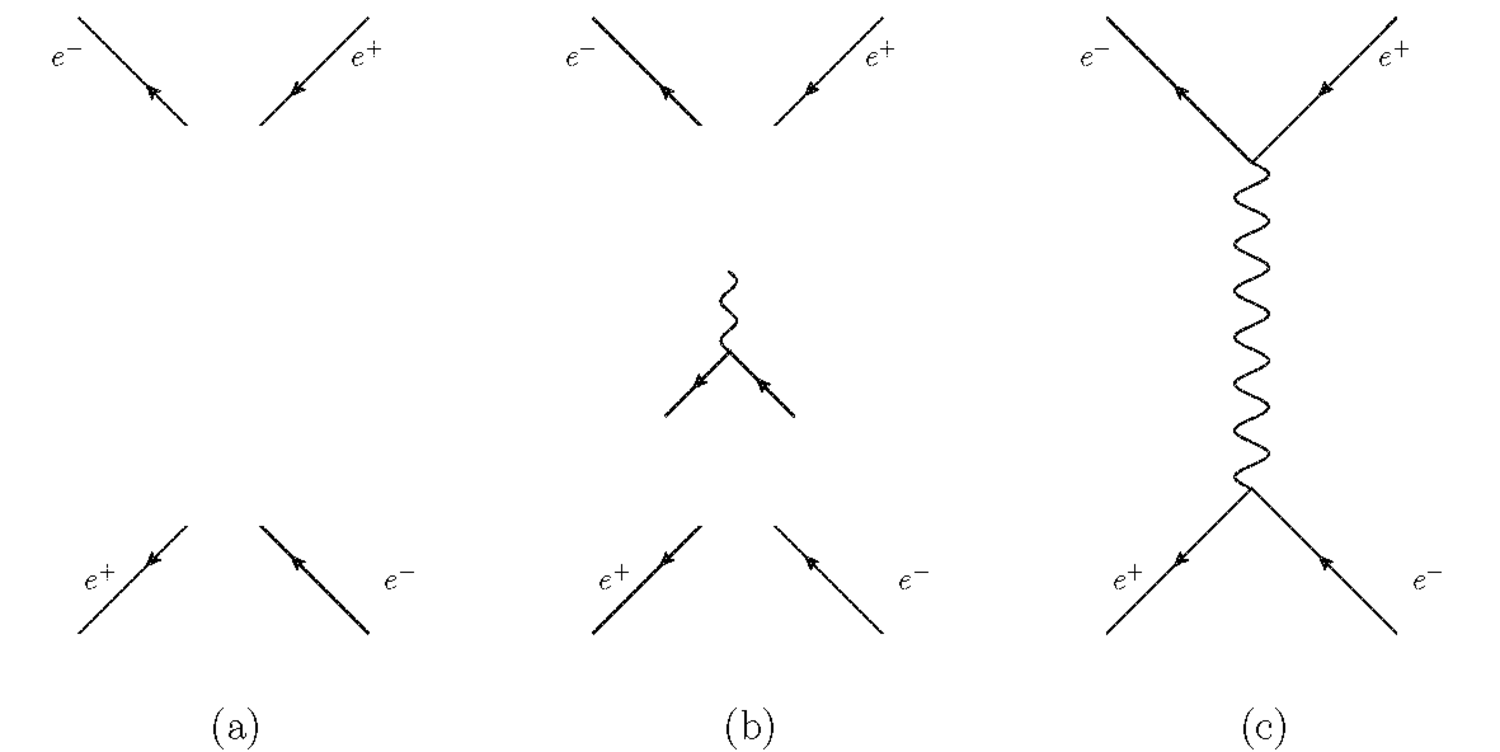
Fig. 11.1: The modern application of Feynman diagrams.
The fundamental element of a quantum electrodynamic interaction is the absorption and emission of a light-quantum by an electron or a positron, which is represented by a point in which two solid lines and a wavy line end or start, see fig. (11.1(b)). Two such elementary interactions suffice to bring about the interaction in this example, see fig. (11.1(c)). Other diagrams, most of them more complex, would complete the representation of the elastic scattering of an electron and a positron using Feynman diagrams.
The numerical value for the reaction rate is obtained by translating the Feynman diagrams into mathematical expressions according to the so-called Feynman rules. In fig. (11.2), we see how Michael E. Peskin and Daniel V. Schroeder show, in their 1995 textbook, what graphical element corresponds to what mathematical expression (Peskin and Schroeder 1995).
While most of the authors on Feynman diagrams warn us of incorrectly interpreting the diagrams in terms of, for instance, particle trajectories, some of them go further and deny any physical interpretation whatsoever. James Robert Brown, for example, maintains such a position and claims: “We see the lines in the diagram; we do not visualize the physical process itself, nor any sort of abstract version of it” (Brown 1996, 267).
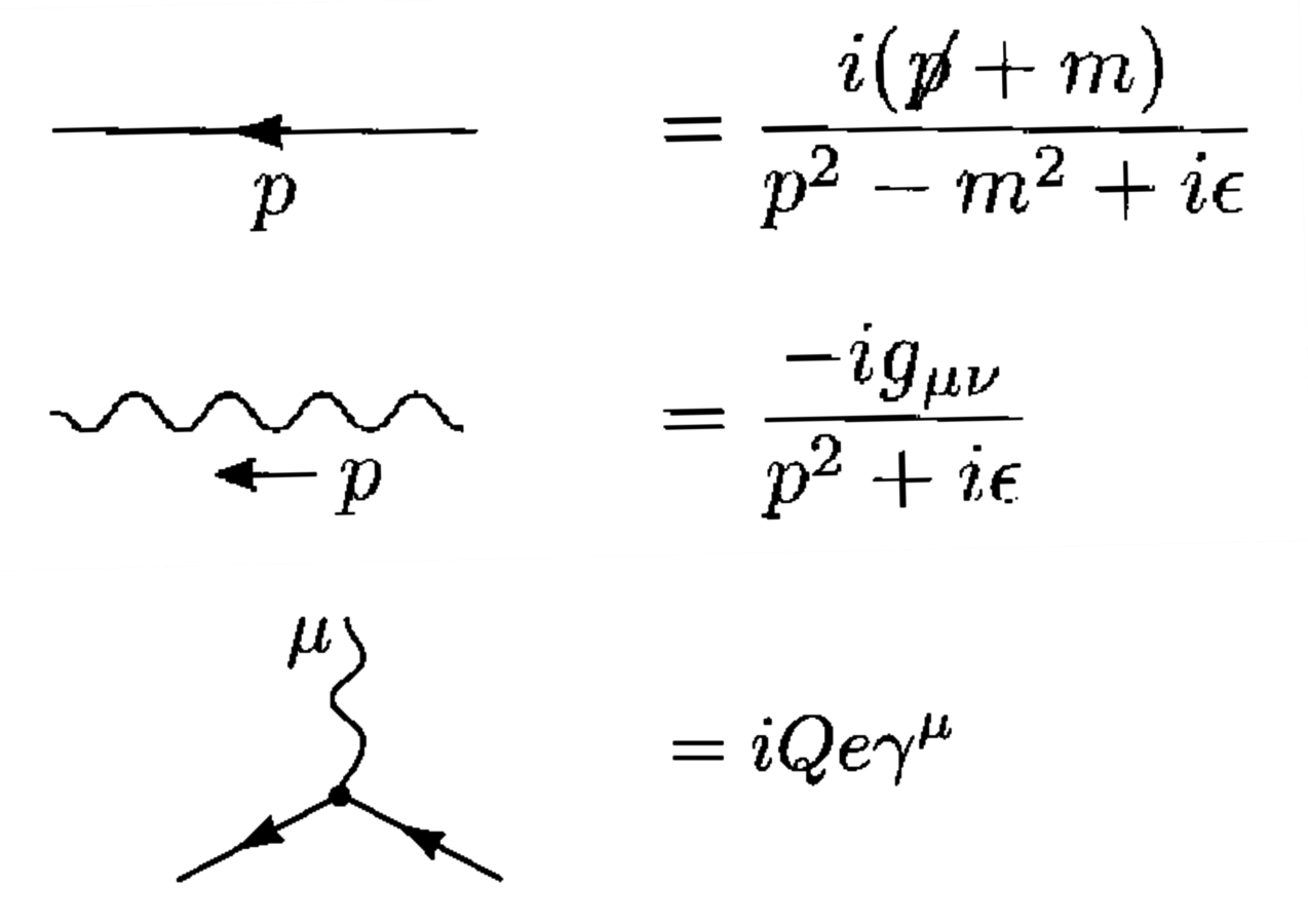
Fig. 11.2: The Feynman rules as presented in Peskin and Schroeder (1995, 801–802).
The view that Feynman diagrams are simply a tool for organizing calculations and the many warnings against making incorrect interpretations also have a bearing on accounts of their origin. Several authors claim that the diagrams were developed to find abbreviations for complicated mathematical expressions. Silvan Schweber says that “[Feynman] diagrams evolved as a shorthand to help Feynman translate his integral-over-path perturbative expansions into the expressions for transition matrix elements being calculated” (Schweber 1994, 434). Brown also suggests that the diagrams are the result of Feynman’s attempts to simplify the task of finding and organizing terms in complicated perturbative calculations: “When Richard Feynman was working on quantum electrodynamics in the late 1940s, he created a set of diagrams to keep track of the monster calculations that were required” (Brown 1996, 265).
Most authors reconstruct the route that led Feynman to devise his new method of diagrams according to the premise that the physical content of the theory remained the same throughout the development. Also, when it comes to evaluating what was achieved, most authors maintain that no changes have occurred, as far as the physics is concerned, either in Feynman’s or in related work by Julian Schwinger and Sin-Itiro Tomonaga. Dyson, who was one of the main actors in their development, would say in 1965:
Tomonaga, Schwinger, and Feynman rescued the theory without making any radical innovations. Their victory was a victory of conservatism. They kept the physical basis of the theory precisely as it had been laid down by Dirac, and only changed the mathematical superstructure. (Dyson 1965, 589)
From a closer study of Feynman’s unpublished manuscripts and early publications, this view of the development and interpretation of Feynman diagrams does not quite fit what emerges as Feynman’s main concern. Feynman almost always used diagrams as a calculational tool and also as a means to represent the physical model by which he interpreted the theoretical equations.
If one is willing to accept that diagrams can have the two functions of calculating and representing at the same time, one could gain further insight into the development of quantum electrodynamics—not only in Feynman’s work, but also beyond it. The differences in the means of representation in use at different stages of the development reflect differences in calculational techniques; in addition, they reflect profound differences in the way quantum electrodynamic phenomena were conceptualized.
In fig. (11.3), we see three examples of processes which are, on the one hand represented by variations of atomic term schemes (left column) and, on the other hand, by a Feynman diagram (right column). The three processes are light- by-light scattering, the Compton effect and the scattering of an electron off an external electromagnetic potential. The use of Feynman diagrams is associated with different, often much more effective ways of calculating. With Feynman diagrams, one often does not need to distinguish between mathematical terms; without Feynman diagrams, those terms have to be treated separately. Without Feynman diagrams, the procedure was, therefore, more complicated and error-prone (Weinberg 1995, 37; Halzen and Martin 1984, 99).
However, the way of calculating was not the only difference that came with the use of Feynman diagrams. Without Feynman diagrams, the phenomena were represented as transitions between energy levels, almost like in traditional atomic physics, as we can see in the top row of fig. (11.3). With Feynman diagrams, see bottom row of fig. (11.3), the phenomena were analyzed into a succession of free propagation of initial quanta which are annihilated when intermediate quanta are created, and those then also get annihilated when the final state quanta are created.
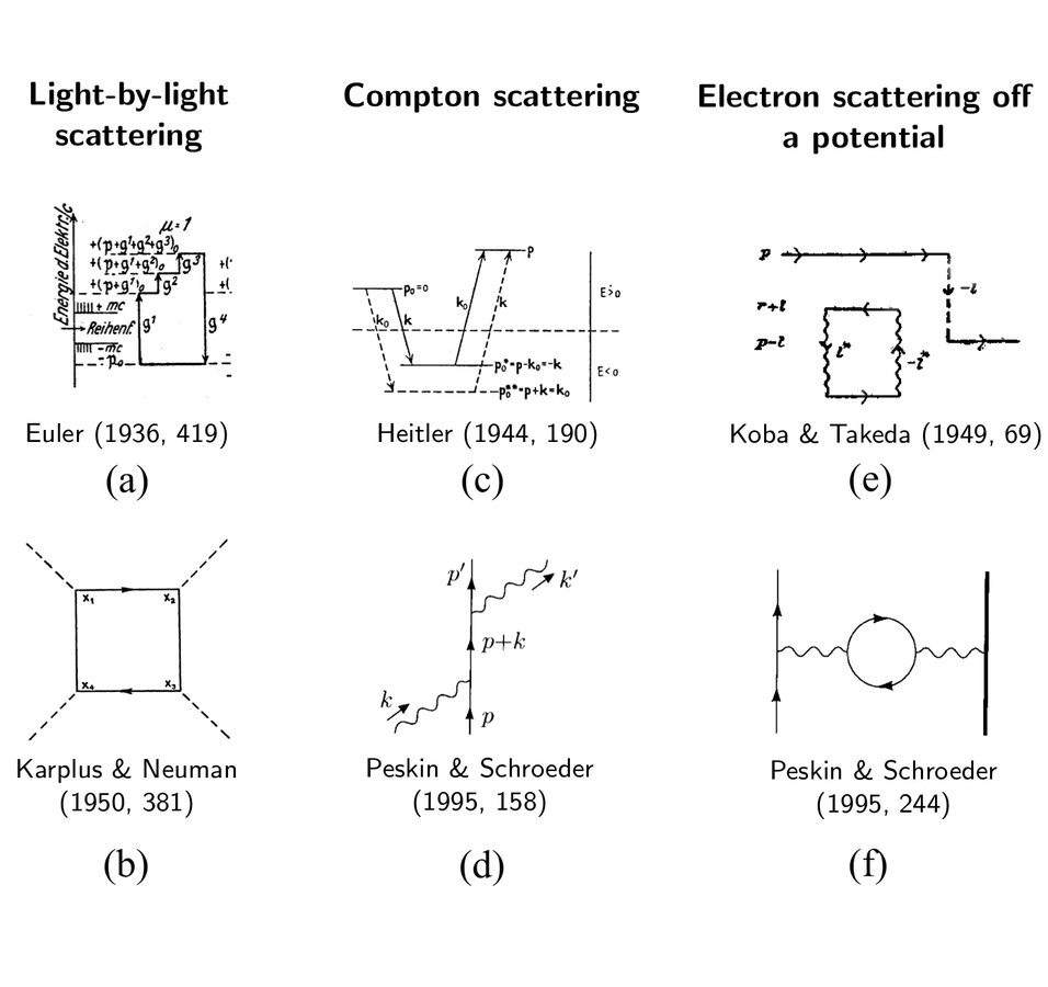
Fig. 11.3: Comparison of representations of elementary particle interactions with Feynman diagrams (lower row) and without Feynman diagrams (upper row). The two diagrams in the first column represent light-by-light scattering; the two diagrams in the second column represent Compton scattering; and the two diagrams in the third column represent the scattering of an electron off a potential. Diagram (a) is a detail from (Euler 1936, 419); (b) is from (Karplus and Neuman 1950, 381); (c) from (Heitler 1944, 190); (d) from (Peskin and Schroeder 1995, 158); (e) from (Koba and Takeda 1949, 69); and (f) from (Peskin and Schroeder 1995, 244). In the third edition of Heitler’s Quantum Theory of Radiation from 1954, the diagram for Compton scattering reproduced here is absent.
11.2 Feynman’s Struggle for a Physical Interpretation
of the Dirac Equation
In my account of the origin of Feynman diagrams, Feynman’s preoccupation with complicated mathematical expressions recedes, while his efforts to develop an appropriate way of representing quantum electrodynamic phenomena comes to the fore. Other accounts, such as Brown’s and Schweber’s, tend to neglect the latter in favor of the former. According to my reconstruction, Feynman diagrams are the final result of Feynman’s quest for an informative physical interpretation of Dirac’s well-known equation. Unpublished manuscripts indicate that Feynman began to seriously “struggle” with the Dirac equation in 1947.
In a letter to his student and friend Theodore Welton, Feynman announced a private research project:2
I am engaged now in a general program of study—I want to understand (not just in a mathematical way) the ideas in all branches of theor. physics. As you know I am now struggling with the Dirac Eqn.
Dirac’s equation had been well known and long-used. What was Feynman looking for? It was not a new version of the equation nor a new method of solution. It was, rather, a deeper understanding of the equation:
The reason I am so slow is not that I do not know what the correct equations, in integral or differential form are (Dirac tells me) but rather that I would like to understand these equations from as many points of view as possible. So I do it in 1, 2, 3 & 4 dimensions with different assumptions etc.3
Clearly, for Feynman, the search for a deeper understanding should lead to an appropriate representation of the phenomena which are described by the equation. The physical interpretation which comes along with the representation should then provide the grounds for circumventing problematic consequences of the equation:
Of course, the hope is that a slight modification of one of the pictures will straighten out some of the present troubles.
The “troubles” were that the Dirac equation yielded empirically well-confirmed predictions when it was applied in a rough approximation (perturbative expansion to the first order). However, when physicists attempted to obtain yet more accurate results by applying the equation in a more rigorous approximation (perturbative expansion to higher orders), the predictions became less precise and completely unusable and uninterpretable: they turned out to be infinite.
11.3 Zitterbewegung
Although part of the material on which my reconstruction of the development of Feynman diagrams is based has previously been analyzed by other scholars, I hope to be able to emphasize more clearly that Feynman’s visualizations were not only a source of inspiration, and what he represented was far more than “toy models” for academic exercises.
In 1947, Feynman began to elaborate on the physical interpretation of Dirac’s equation as describing a Zitterbewegung, a quivering motion, of the electron, which both Gregory Breit (1928) and Erwin Schrödinger (1930) had proposed.4 Breit considered an electron in an electromagnetic field while Schrödinger only considered the case of no forces. In either the one or the other form, the interpretation of the Dirac equation as describing a Zitterbewegung must have been well-known since it had been published in influential journals and was discussed in Dirac’s book The Principle of Quantum Mechanics (Dirac 1935) and in his Nobel lecture (Dirac 1933).
In his investigations, Feynman restricted himself, most of the time, to the one-dimensional version of the equation. From the Hamiltonian which corresponded to the one-dimensional Dirac equation for an electron in an electromagnetic field

|
11.1 |
Feynman deduced that, according to Dirac’s equation, the instantaneous velocity of the electron always equaled the speed of light. This was no novel result, however, since it was discussed in Breit’s, Schrödinger’s and other aforementioned publications.
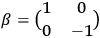
In the above eq. (11.1), the electron’s wave function
 has two components;
 and
and
 are constant
matrices:
are constant
matrices:
 ,
,
 , and the momentum
 is defined as the
operator of partial differentiation with respect to the spatial variable
is defined as the
operator of partial differentiation with respect to the spatial variable
 , that is,
 .
.
 and
and
 are,
respectively, the scalar and the vector potential of the electromagnetic
field;
are,
respectively, the scalar and the vector potential of the electromagnetic
field;
 is the mass of the electron.5
The result that the electron’s speed was always identical to that of light
meant, in Feynman’s notation and units, that the velocity operator
 equaled the two-by-two Dirac matrix
 . To derive this result,
Feynman used the familiar relationship between the total time derivative
(
. To derive this result,
Feynman used the familiar relationship between the total time derivative
(
 ) of any operator (
 ) and its commutator with the Hamiltonian
operator (
) and its commutator with the Hamiltonian
operator (
 ) and the partial temporal derivative (
 ) of the operator:
 .
.
The result is puzzling at first since it seems to contradict the fact that no massive particle is known which moves at the speed of light. Also, the theory of special relativity precludes the existence of such a particle because, according to relativistic laws, the particle would contain an infinite amount of energy.
In Breit’s and Schroedinger’s publications, as well as in Dirac’s book and Nobel lecture, the apparent contradiction to the empirical observations was resolved: we are dealing with a Zitterbewegung, a quivering motion, of the electron of which we can only observe the displacements on average. Thus, although the instantaneous velocity is the speed of light, the observable velocity is finite.
Feynman tried to incorporate this interpretation into his earlier work on an alternative formulation of non-relativistic quantum mechanics. In that work, Feynman had attempted to eliminate the divergences associated with self-interactions of the particles by representing the time development of the wave-function in terms of the action. The most important results of that work are published in an article in the Reviews of Modern Physics (Feynman 1948a). However, to a large extent, he had already obtained these results in 1942 in his doctoral thesis, which has been published only recently (Feynman 2005). In these two publications, Feynman showed explicitly that the time evolution of the wave-function was given by the sum of contributions of all paths that led a particle from its initial to its final position. The contribution of any one path was given by the action evaluated along that path.
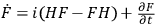
In his unpublished notes from 1947, the first problem he tackled was
that no justifiable expression for the action was known at the time.
Therefore, Feynman considered a lattice of one space and one time dimension
and interpreted the two components of Dirac’s wave function as describing a
particle that traveled either to the right or to the left. Feynman graphically
represented a special case of the situation in a diagram. In this special
case, the initial wave function of the particle has only a “right”
component, and Feynman wants to determine the “left” component at the
lattice point
 which was
 lattice spacings
 away in one
diagonal direction, and
away in one
diagonal direction, and
 lattice spacings in the other diagonal direction.
Through a change of variables and an iterative solution procedure, Feynman
deduced a factor
 by which to count each reversal in the direction
of the particle. The problem of finding the action thus came to working
out how many paths there were that had a given number of changes in
direction.6
by which to count each reversal in the direction
of the particle. The problem of finding the action thus came to working
out how many paths there were that had a given number of changes in
direction.6
He could then count each change by a factor
 and sum over all
paths. The obtained expression thus determined the time evolution of
the wave-function exactly as the action would do.
and sum over all
paths. The obtained expression thus determined the time evolution of
the wave-function exactly as the action would do.
Fig. 11.4: Abstract graphical representation of the quivering electron, which Feynman used for counting the number of possible zigzag paths. Reproduced by the author from a manuscript page by Feynman probably dating from 1947, see (Wüthrich 2010, 69).
Feynman thus solved the Dirac equation by “path counting,” as he wrote in his notes. Actually, by counting the zigzag paths he obtained the Green’s function associated with Dirac’s equation, which Feynman mentioned in passing on the same manuscript page from which fig. (11.4) is reproduced.
11.4 Positrons and Interaction
One of the striking features of the Dirac equation was its implication, or at least suggestion, of the existence of antiparticles. Feynman had not yet taken this into account, as far his “struggle” with the Dirac equation was concerned. Maybe he had an uneasy sense of the difficulties which would arise in the application of his method of path-counting to those positrons.
Taking an idea that John A. Wheeler, his PhD supervisor, had communicated to him in the autumn of 1940, Feynman conceived of the positron as an electron moving backward in time.7 In my sketch of the modern application of Feynman diagrams, I briefly mentioned that such a conception is still in use with Feynman diagrams. For Feynman’s model of the quivering electron and its possible paths, this meant that he now also had to account for loops of a path. The presence of electrons moving backward in time opened up the possibility of paths going through the same point twice, forming loops. The undesirable consequence of this was that now an infinite number of paths were possible between a given initial and a given final position, even though Feynman considered a space-time lattice and not a continuum. Therefore, the path-counting amounted to an infinite series which did not seem to converge, and the method seemed inapplicable.
However, in his notes, Feynman recognized that the possibility of a path that contained a loop implied the possibility of a path that contained the same loop but went through it in the opposite direction. Moreover, the contributions of the two paths canceled each other out, and Feynman concluded that “any completely closed loop cancel[ed].”8 Therefore, paths containing loops could be dismissed, and the method of path-counting was saved.
After having successfully dealt with positrons, Feynman moved to the next problematic issue. He attempted to incorporate the interaction between two or more particles into his model system of the Dirac equation. To this end, he tried to construct a Hamiltonian operator out of the action function which he had used, together with Wheeler, in his alternative formulation of classical electrodynamics (Wheeler and Feynman 1949).9
However, unlike with the incorporation of positrons, the difficulties were
insurmountable. He was only able to treat the special case of an interaction
which vanished after a certain time. In his notes, he expressed his
dissatisfaction with this state of affairs. Of his attempts to describe a
system of two particles by a joint wave function
 he says:
It is a bit hard to see how to definefor path pair
and
, since there are some terms from interaction at
from
which is unspecified. However if the interaction is zero beyond
we are OK. Hence, at present, I can only specify
for paths which are long enough that they go beyond the time of interaction (this stinks).10
11.5 Abandoning the Search for a Microscopic Analysis
Because he was not able to satisfactorily incorporate the interaction of particles into the model of the quivering electron, Feynman abandoned it. To him, it seemed impossible to analyze interacting electrons and positrons in terms of the microscopic Zitterbewegung implied by Dirac’s equation. However, a closer inspection of his published papers (Feynman 1949a; 1949b) shows that he did not give up the attempt to construct a model system of the Dirac equation altogether. Only the level of specification of his explanatory model was about to change. Up to that moment, he had analyzed the propagation of an electron by a superposition of microscopic zigzag paths. This had led to a description of the propagation by a Green’s function. Afterward, Feynman would work directly on this less-specific level of Green’s functions and leave the propagation of the electron from one point to another without further analysis.
In this way, Feynman eventually succeeded in adequately describing the interaction between two electric particles. To obtain such a description, he took the classical mathematical expression for the potential as a basis. However, unlike in his previous unsuccessful attempt to incorporate interactions, he did not attempt to construct a quantum description by a Hamiltonian operator out of the classical expressions. In the previous attempt, he had needed the Hamiltonian to describe the quivering motion of the interacting particles. This time, he left aside the quivering motion and tried to fit the classical expressions into his more coarse-grained model of propagating particles described by Green’s functions.
Feynman was probably more prepared than other physicists to interpret the electromagnetic interaction as being brought about by emission and absorption of light quanta because, in his “cut-off” paper (Feynman 1948b, 1431), he saw a way to avoid the difficulties, related to the polarization of the light quanta, which such an interpretation usually had to face. After some modifications of the classical potential, which put the expression for the potential side by side with the Green’s functions that described the propagation of the electrons and positrons, the interpretation of the potential as describing the propagation of a light quantum must, therefore, have seemed natural to him.11
This reinterpretation is clearly visible in the graphical representation Feynman used at that time, compared to the one he had used in the earlier work with Wheeler, see fig. (11.5), upon which his previous attempt to adequately describe interactions had been based.

Fig. 11.5: Graphical representation of the electromagnetic interaction between two particles (a) in Wheeler’s and Feynman’s alternative classical electrodynamics (Wheeler and Feynman 1949, 431) and (b) in Feynman’s approach to quantum electrodynamics (Feynman 1949b, 772).
Feynman thus achieved a description of the time evolution of a quantum electrodynamic system, including interaction, by Green’s functions describing the free propagation of electrons, positrons and photons. This marks the endpoint of Feynman’s contributions in the period covered by this reconstruction of the genesis of Feynman diagrams. However, to understand how the modern form and use of Feynman diagrams came about, we cannot stop here. The modern form and use of Feynman diagrams goes back not only to the diagrams Feynman left us in his “space-time approach” (Feynman 1949b), rather, to a considerable extent, it goes back to what Dyson made of them in the context of the quantum field theory of the time. I address Dyson’s contributions (Dyson 1949a; 1949b) in the next section.
11.6 Solution to the Problems through an Appropriate
Representation of the Phenomena
With the innovative interpretation of the classical interaction as a propagation of a light quantum, Feynman fulfilled his aspiration, which he had announced in his letter to Welton (see footnote 2), to find a “picture,” the “slight modification” of which would remove the theory’s problematic infinities. He had now reduced all QED processes to the free propagation of initial quanta which are annihilated when intermediate quanta are created, these also get annihilated when the final state quanta are created. All QED processes were seen to be composed of a fundamental process: the emission or absorption of a light quantum by an electron or a positron described as a sequence of propagation of the particles and the quantum. Feynman had thus found what he had been looking for ever since he began his “struggle” to fully understand the Dirac equation: a means of representation that made explicit which features of the theory could be held responsible for its divergence problems. If all phenomena the theory of QED described were essentially made up of one fundamental process, an appropriate modification of the representation of this process should suffice to eliminate the problems.
The community of physicists working at the time skeptically received Feynman’s modified theory of QED, with which Feynman intended to solve the problems of the then-current theory, and they had a hard time understanding what it was all about. However, the main reason for the skeptical attitude of most physicists was not Feynman’s extensive use of diagrams but rather the obsolete theoretical principles on which Feynman had based his theory. For instance, Feynman understood that, as in quantum mechanics, wave functions are probability amplitudes for the position of a particle. However, the theory of QED of the time was a theory in which the wave function was replaced with an operator-valued field, the quanta of which are electrons and positrons.
It was Dyson who rescued Feynman’s diagrams from their obsolete theoretical setting. He began to interpret them in the context of 1940s state-of-the-art quantum field theory and eventually brought them to fruition. Dyson showed, for instance, that Feynman’s Green’s functions corresponded to quantum-field-theoretical vacuum expectation values (Dyson 1949a, 494). Thanks to the theoretical updating, Dyson could eliminate the problematic divergences in a more systematic manner than Feynman, and to arbitrary high orders in perturbation theory (Dyson 1949b).
Dyson showed that problematic divergences arose from two types of basic processes, which he represented graphically as shown in fig. (11.6(a)) and fig. (11.6(b)). To precisely determine observable quantities like cross sections and reaction rates, one should take all combinations of these processes into account, such as the one shown in fig. (11.6(c)).

Fig. 11.6: (a) and (b) show the two basic types of processes which are responsible for the problematic divergences according to Dyson’s analysis (Dyson 1949b, 1741–1742); (c) shows a combination of the two; (d) the corresponding “irreducible graph” (drawings (c) and (d) by the author).
However, Dyson was able to show how one could dispense with all of these problematic processes. He modified the Green’s functions (or vacuum expectation values) which describe the free propagation of the field quanta and the operator which occurs in the description of the interaction, such that only “irreducible graphs” (Dyson 1949b, 1743), like the one which is shown in fig. (11.6(d)), have to be taken into account.
Dyson (1949b, 1754–1755) argued that the infinities arose from an over-idealized description of the interaction. The problematic diagrams represented effects that are entirely unobservable since they represented inevitable fluctuation processes. In the quantitative evaluation of the irreducible graphs, the infinite factors appeared only in combinations which could be interpreted as an effective mass and charge. The different types of divergences could thus be calibrated against each other such that only the observed values for the mass and charge appeared in the observable quantities. This method came to be known as renormalization.
Dyson was surprised by the ease with which the recalcitrant problems concerning the divergences could be eliminated. For him, the cancellation of the infinities to yield the finite observable quantities was a physical fact:
The surprising feature of the [theory] as outlined in this paper, is its success in avoiding difficulties. Starting from the methods of Tomonaga, Schwinger and Feynman, and using no new ideas or techniques, one arrives at an S matrix from which the well-known divergences seem to have eliminated themselves. This automatic disappearance of the divergences is an empirical fact, which must be given due weight in considering the future prospects of electrodynamics. (Dyson 1949b, 1754)
The apparent simplicity of the solution can, at least partially, be explained by Dyson’s use of an appropriate representation suggested by Feynman. Feynman’s representation identified exactly the right elements to eliminate the divergences in a systematic and physically interpretable manner. Once Feynman had provided the appropriate representation, the successful modification of the theory, as performed by Dyson, no longer involved fundamental revisions but certainly deep insights as to the consequences of the new way of representing the phenomena. The development of an appropriate means of representation by Feynman was the fundamental, though not yet complete, revision Dyson successfully put to use.
11.7 Comparison to Other Developments of Concepts and Means
of Representation
The early history of Feynman diagrams lends itself to a comparison with other developments of concepts and means of representation, in particular to James Clark Maxwell’s abandonment of the mechanical model (Siegel 1991) and to medieval representations of change (Schemmel 2010).12 I close my contribution with a short sketch of what seem to be the most interesting similarities and differences, with respect to the aforementioned cases, worthwhile to pursue further.
11.7.1 Maxwell’s Abandonment of the Mechanical Model
According to Daniel Siegel, Maxwell interpreted his mechanical vortex model for electromagnetic phenomena more realistically than most of the scholarship on Maxwell would acknowledge. In the years following 1862, however, Maxwell partially abandoned the model and aimed to formulate his theory on the displacement current and light without a full commitment to the model which initially provided much of the necessary insights to the construction of the theory. Similarly, Feynman’s move from the representation of the quivering electron to the representation of the electron’s and positron’s propagation by Green’s functions is an abstraction of a theoretical description from some of the features the object under consideration was, up to then, assumed to have.
I would emphasize, however, that Feynman did not thereby abandon the physical interpretation of the diagrams; only the level of specification of the representation changed. To what extent this would also be true of Maxwell’s case I am not able to assess, and it is not clear to me how much Siegel would endorse such a view. But it seems plausible that Maxwell’s progress was also a process of changing the level of specification of the representation without giving up the physical interpretation of his equations.
11.7.2 Medieval Representations of Change
According to Matthias Schemmel (2010), the medieval representations of change were an essential ingredient for the development of an appropriate concept of velocity when early modern scientists, like Thomas Harriott, employed them in their investigations. The form of the diagrams remained nearly unchanged while their interpretation was significantly revised.
Two phases of the development of Feynman diagrams show similar characteristics. Hans Euler, Walter Heitler, and Zirô Koba and Gyô Takeda used traditional means to represent phenomena, which they described using novel concepts. In traditional term schemes, the horizontal lines represented stable energy levels which manifested themselves as lines in spectroscopic analyses. In the hands of Euler and others, these horizontal lines indicated, instead, energy levels of electrons and positrons which were never observed. They represented intermediate states in a process in which only the initial and final states were observable.
The other phase in which the diagrams hardly changed but their interpretation did was the systematization of Feynman’s theory by Dyson. With Feynman, the diagrams operated in the context of quantum mechanics, which describes particles by a wave-function. With Dyson’s systematization, the context is quantum field theory, which describes particles as quanta of fields. With Feynman, the lines in the diagrams represented particle propagators, while with Dyson, the lines represented vacuum expectation values of field operators.
The most significant conceptual change, however, occurred with the invention of Feynman’s diagrams during his search for an adequate interpretation of Dirac’s equation. Compared to the traditional means of representing QED phenomena by adaptations of term schemes, Feynman’s diagrams differ significantly, both in their form and in their interpretation. Instead of horizontal lines as main graphical elements, we have lines and vertices. Instead of transitions between energy levels, we have propagation of particles.
Rather than catalysts which stimulate a conceptual development but remain unchanged, as in the case Schemmel describes, the Feynman diagrams are a product of a process in which both the graphical means of representation and the conceptual framework were developed at the same time. It is hard to distinguish the process of conceptual development and the development of appropriate means of representation. The genesis of Feynman diagrams is a case in point to show that conceptual developments are carried out through a concrete manipulation of graphical means of representation.
Abbreviations and Archives
| Caltech Archives | Archives of the California Institute of Technology, Pasadena, CA |
| Niels Bohr Library & Archives | American Institute of Physics, College Park, MD, USA |
Acknowledgements
I am grateful to the Max Planck Institute for the History of Science, Berlin for the generous travel stipend for junior scholars for participation in the conference, and to Shaul Katzir and an anonymous referee for valuable comments. The research for my PhD thesis on the genesis and interpretation of Feynman diagrams has been funded by the Swiss National Science Foundation (grant no. 100011–113589), supervised by Gerd Graßhoff and co-refereed by Tilman Sauer.
References
Breit, Gregory (1928). An Interpretation of Dirac's Theory of the Electron. Proceedings of the National Academy of Sciences of the United States of America 14: 553-559
Brown, James R. (1996). Illustration and Interference. In: Picturing Knowledge: Historical and Philosophical Problems Concerning the Use of Art in Science Ed. by Brian S. Baigrie. Toronto: University of Toronto Press 250-268
Dirac, Paul A. M. (1928). The Quantum Theory of the Electron. Proceedings of the Royal Society A 117: 610-624
- (1935). The Principles of Quantum Mechanics. Oxford: Clarendon Press.
Dyson, Freeman J. (1949a). The Radiation Theories of Tomonaga, Schwinger, and Feynman. Physical Review 75: 486-502
- (1949b). The S-Matrix in Quantum Electrodynamics. Physical Review 75: 1736-1755
- (1965). Tomonaga, Schwinger, and Feynman Awarded Nobel Prize for Physics. Science 150: 588-589
Euler, Hans (1936). Über die Streuung von Licht nach der Diracschen Theorie. Annalen der Physik 418: 398-448
Feynman, Richard P. (1948a). Space-Time Approach to Non-Relativistic Quantum Mechanics. Reviews of Modern Physics 20: 367-387
- (1948b). Relativistic Cut-Off for Quantum Electrodynamics. Physical Review 74: 1430-1438
- (1949a). The Theory of Positrons. Physical Review 76: 749-759
- (1949b). Space-Time Approach to Quantum Electrodynamics. Physical Review 76: 769-789
- (1966). The Development of the Space-Time View of Quantum Electrodynamics. Science 153: 699-708
- (2005). The Principle of Least Action in Quantum Mechanics. In: Feynman's Thesis: A New Approach to Quantum Theory Ed. by Laurie M. Brown. Singapore: World Scientific Publishing 1-69
Fock, Vladimir (1929). Über den Begriff der Geschwindigkeit in der Diracschen Theorie des Elektrons. Zeitschrift für Physik 55: 127-140
Halzen, Francis, Alan D. Martin (1984). Quarks and Leptons: An Introductory Course in Modern Particle Physics. New York: John WileySons.
Heitler, Walter (1944). Quantum Theory of Radiation. London: Oxford University Press.
Karplus, Robert, Maurice Neuman (1950). Non-Linear Interactions between Electromagnetic Fields. Physical Review 80: 380-385
Koba, Zirô, Gyô Takeda (1949). Radiation Reaction in Collision Process III: First Radiative Correction for an Arbitrary Process Including Electrons, Positrons, and Light Quanta. Progress of Theoretical Physics 4: 60-70
Peskin, Michael E., Daniel V. Schroeder (1995). An Introduction to Quantum Field Theory. Boulder (Colorado): Westview Press.
Schemmel, Matthias (2010). Medieval Representations of Change and Their Early Modern Application. Berlin: Max Planck Institute for the History of Science.
Schrödinger, Erwin (1930). Über die kräftefreie Bewegung in der relativistischen Quantenmechanik. Sonderausgabe aus den Sitzungsberichten der Preußischen Akademie der Wissenschaften Phys.-Math. Klasse 24: 418-428
Schweber, Silvan S. (1986). Feynman and the Visualization of Space-Time Processes. Reviews of Modern Physics 58: 449-508
- (1994). QED and the Men Who Made It: Dyson, Feynman, Schwinger, and Tomonaga. Princeton (NJ): Princeton University Press.
Siegel, Daniel M. (1991). Innovation in Maxwell's Electromagnetic Theory: Molecular Vortices, Displacement Current, and Light. Cambridge: Cambridge University Press.
Weinberg, Steven (1995). The Quantum Theory of Fields. Cambridge: Cambridge University Press.
Wheeler, John A., Richard P. Feynman (1949). Classical Electrodynamics in Terms of Direct Interparticle Action. Reviews of Modern Physics 21: 425-433
Wüthrich, Adrian (2010). The Genesis of Feynman Diagrams. Dordrecht: Springer.
Footnotes
A more detailed account of what is described in sects. (11.1) to (11.6) can be found in (Wüthrich 2010). Some passages and figures from that publication are reproduced here with kind permission of Springer Science and Business Media.
The following three quotations are taken from Richard Feynman’s 1947 letter to Theodore Welton, in “Papers of Richard Phillips Feynman," California Institute of Technology (Caltech) Archives, Box 11, Folder 2. Partially reproduced in (Wüthrich 2010, 83–95). See also (Schweber 1994, 406–408).
The italicized word is underlined in the original letter.
For details and a facsimile of the manuscript page (Caltech Archives, Box 11, Folder 2), see (Wüthrich 2010, 66–68).
For details and a facsimile of the manuscript page (Caltech Archives, Box 11, Folder 2), see (Wüthrich 2010, 68–75).
For details of how Feynman learned about Wheeler’s idea, see (Schweber 1986, 460; 1994, 387–388; Feynman 1966, 702, 705–706). See also Charles Weiner’s Interviews with Dr. Richard Feynman, 4 March to 28 June 1966, vol. 2, p. 32, in Niels Bohr Library & Archives.
For a facsimile of the page in question, (Caltech Archives, Box 12, Folder 9), see (Wüthrich 2010, 97; Schweber 1986, 482).
For details, see (Wüthrich 2010, 104–108).
Caltech Archives, Box 11, Folder 2. For a facsimile, see (Wüthrich 2010, 110).
For details, see (Wüthrich 2010, 133–136).
I thank Shaul Katzir and Jürgen Renn for having suggested these comparisons.