Research in quantum physics began in Europe and then spread to many parts of the world. Outside Europe and North America, Japan was one of the places where quantum physics research successfully took off before World War II. Although Japan started absorbing European scientific knowledge in the 18th century,1 modernized educational and research institutions for the sciences appeared only in the late 19th century, after the so-called Meiji Restoration. Nevertheless, in the late 1920s, Japanese physicists began producing first-rate theoretical research,2 and in 1935, Yukawa Hideki published his Nobel Prize-winning work on meson theory (Yukawa 1935).
How could this happen? Answering this would be of some importance for understanding the spread of quantum physics worldwide, or more generally for understanding the global dissemination of modern science in the 20th century. Unless we believe in the teleologically driven dissemination of science, it requires an explanation why other, vastly different cultures came to adopt European science. Instead of giving a full answer to the question of dissemination of quantum physics, which I will attempt in a separate and much larger work, in this paper I will show a possible link between preexisting conditions in Japan and the introduction of quantum physics. The main goal is to identify one possible aspect of these conditions that eased the introduction of quantum physical research into Japan: electrical engineering.
Nishina Yoshio3 (1890–1951) was among the first generation of Japanese quantum physicists who produced noteworthy theoretical research in quantum physics. He established himself as a physicist while staying in Europe, in particular Copenhagen, and in collaboration with Oskar Klein, carried out significant theoretical work on quantum physics, resulting in the Klein-Nishina formula (Klein and Nishina 1929).4 After his return to Japan in late 1928, he introduced quantum mechanics there. He became a leading figure in this field in Japan, paving the way for other Japanese physicists.5
Curiously, Nishina was originally trained as an electrical engineer, not a physicist. When he entered the Sixth Higher School in Okayama at the age of 20 in 1910, he chose engineering as his major.6 Later he advanced to the Department of Electrical Engineering at Tokyo Imperial University in 1914. It was only after his graduation and employment at the Institute for Physical and Chemical Research (RIKEN) that he changed his career to physics. RIKEN allowed him to study abroad, from 1921 to December 1928. His stay in Europe during this period definitively made Nishina a quantum physicist.
Becoming a quantum physicist from Japan must have been difficult enough. How could Nishina move across, not only the cultural boundary between Japan and Europe, but also the disciplinary boundary between electrical engineering and physics? In an attempt to develop a partial answer to this question, I ask: Did the electrical engineering training that Nishina received prepare him for research in quantum mechanics?
A late-comer to the industrialized world, Japanese society prioritized practical subjects such as electrical engineering. These training fields may have provided intellectual resources and institutional bases that helped motivate, legitimize and sustain quantum physical research. The goal of this paper is to explore such possible links between electrical engineering training and theoretical practices of quantum mechanics in the local Japanese context to understand how new theoretical scientific practices traveled across cultures.
The role of an engineering background in the development of physics practices has been studied in several cases, including Albert Einstein, Henri Poincaré and Julian Schwinger (Pyenson 1982; 1985; Galison 1997; 2003). It is not within the scope of this paper to fully study physicists who were involved in engineering research during their training, as a hobby, or in the context of commissioned military research. However, given the topic of this paper, an obvious example for such an investigation is Paul Dirac, who received electrical engineering training in Bristol. In studying Dirac’s engineering training and his wartime engineering work on isotope separation, Richard Dalitz stresses Dirac’s engineering and practical sides and discusses how these could have been integrated into his attitude to physics (Dalitz 1990). Peter Galison (2000) shows how Dirac expressed his ideas in drawings, using a form of projective geometry, which was part of his engineering training, and how these drawings were suppressed in his published papers.
These studies indicate that the relationship between engineering and physics was not a simple deterministic one. In a similar vein, this paper is not an attempt to provide a causal explanation of how socio-cultural or intellectual contexts shaped or influenced the way quantum mechanics was introduced into Japan and how Japanese physicists came to practice quantum physics in a different way. Nor do I claim that Nishina turned to quantum mechanics or carried out specific theoretical research (such as his collaboration with Klein on the Klein-Nishina formula) because of his electrical engineering background. In particular, I need to emphasize that it is not my intention to show that Nishina did theoretical physics differently from other physicists because of his earlier training in electrical engineering. Since the main focus of this paper is work that Nishina and Klein coauthored, such an analysis is out of the question anyway. My goal here is different and more modest. While one could point out various characteristics shared by quantum mechanics and electrical engineering in general terms, this paper aims to point out particular characteristics relevant to the case of Nishina’s engineering training and his specific research in quantum mechanics, and to locate them in the historical context surrounding him. Rather than showing differences, I seek to find out how Nishina came to do things similar to the work of European physicists.
I pay particular attention to details of the mathematical practices in engineering to which Nishina was exposed and accustomed. I explore technical details of electrical engineering and physics to indicate some resemblances between the theoretical practices of the engineering and the quantum physics to which Nishina was exposed and upon which he drew.
7.1 Engineering in Japan
Scrutinizing socio-cultural contexts of physics in Japan is not the purpose of this paper, but a brief description might be helpful. Engineering had higher priority and more prestige than physics in early 20th century Japan. In the process of modernization after the Meiji Restoration, Japan included engineering in its higher education from the very beginning, motivated by the need for engineers to build modern infrastructure, such as telegraphs and railroads. Science was mostly, if not entirely, meant to be a basis for engineering and was taught in schools mainly to prepare engineers (Hirosige 1973; Bartholomew 1989). Hence, it was natural that atomic physics was often identified as a basis of electrical engineering. Physics provided a basic understanding of electricity.
At the same time, the electron was one of the foci of atomic physics as it was introduced into Japan in the early 20th century.7 The result was that there was an emphasis on the theory of the electron in textbook physics. Simultaneously, physicists themselves took advantage of the notoriety of electrons in their popularizing activities. Here, I give three examples for this. The first, Nagaoka Hantarō (1865–1950), known for his Saturnian model of an atom,8 was one of the early Japanese professors of physics at Tokyo Imperial University and the leading Japanese atomic physicist before the introduction of quantum mechanics. His popular book, Genkon no denkigaku (Studies of electricity today) (Nagaoka 1912), is an account of the physics related to electricity, including not just classical electromagnetic theory but also atomic physics, with an obvious focus on the electron.
The second, Mizuno Toshinojō (1862–1944), was a contemporary but less-known physicist at Kyoto Imperial University. While Nagaoka’s activities extended into various areas, Mizuno focused on studies of the electron. His 1912 book, Denshiron (The electron theory), was basically a textbook of atomic physics (Mizuno 1912). More interestingly, his 1918 book, Densi no katsudō (Activities of the electron), was a more popular book, aimed at explaining the recent physics of the electron to a lay audience (Mizuno 1918).
The third example is Aichi Keiichi (1880–1923), another theoretical physicist who worked at Tohoku Imperial University. Known for many highly mathematical works on various topics, he wrote a book entitled Denshi no jijoden: Tsūzoku kagaku kōgi (The autobiography of an electron: A popular science account), a popular account of atomic physics (Aichi 1923). As in Charles Gibson’s The Autobiography of an Electron (1911) published over ten years earlier, the electron takes the role of narrator and describes its properties and roles in nature and society.
Apparently, these physicists tried to gain popular support and interest by using the electron to connect their field to electricity. At the same time, as professors at Japan’s key higher education institutions, they were in a position to teach students, who might seek jobs at electric companies, as well as to teach electromagnetism to future engineers at secondary and tertiary schools.
In light of this context, Nishina’s career appears more cohesive; beginning in his undergraduate years, he mostly studied topics related to the electron. In fact, his elder brother, Nishina Teisaku, described the purpose of Nishina’s long stay in Europe as a study of electricity and assumed that his study would have practical implications for electrical engineering. This was probably the way Nishina justified his study abroad to his family and relatives.9
7.2 Nishina Yoshio as an Engineering Student
The connection between electrical engineering and physics went farther than the fact that both fields dealt with electricity. The theoretical and mathematical aspects of these research areas reveal additional similarities. As a student of electrical engineering, Nishina was immersed in a highly theoretical and mathematical school of electrical engineering under Hō Hidetarō (1872–1931), who was Nishina’s academic advisor at Tokyo Imperial University.
Hō is known as the author of many electrical engineering textbooks, in particular works on alternating current circuits and transition phenomena. He is also known for introducing Charles Proteus Steinmetz’s theory of alternating current (Steinmetz 1893) to Japan.10 He is best known for his work in Japan on the Hō-Thévenin theorem.
Nishina’s disciplinary identity was deeply lodged in the alternating current theory of electrical engineering under the influence of Hō and Steinmetz. In his later years, when asked to discuss the books that inspired him in his youth, Nishina listed four: The Mathematical Theory of Electricity and Magnetism by James Jeans published in 1908, Theory and Calculation of Alternating Current Phenomena by Steinmetz published in 1897, Wechselstromtechnik by Engelbert Arnold published in 1902, and Kōryū riron (Alternating current theory) by Hō published in 1912 (Nishina 1946).11
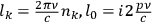
To illustrate the kinds of physical phenomena Hō treated in his textbook, let me summarize one example from his Hadō, shindō oyobi hirai (Wave, vibration and lightning arrester), first published in 1915.12 When electric current flows along an ideal wire (whose resistance and inductance can be ignored), nothing happens. Hō constructed a theory that predicts what happens when there are various kinds of electromagnetic “barriers” along its way. Here, as an example, I take the case of electric current in a sinusoidal (wave-like) form and a coil acting as a “barrier.”
Suppose there is a wire whose inductance and capacitance per length are
 and
and
 respectively, and there is a coil at point
 , whose inductance is
 . The coil is infinitesimally short and can be treated as a point. There are currents in the form of incoming, reflecting and penetrating waves at point
 . Let us say functions
 ,
,
 , and
, and
 are the currents of the incoming, reflecting and penetrating waves. From classical electromagnetic theory, it follows:
|
7.1 |
where
 and
and
 is determined by initial conditions.
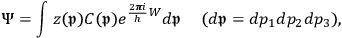
For example, if the incoming wave is a half wavelength of a sinusoidal wave with a certain angular frequency
 :
:
|
7.2 |
the penetrating and reflecting waves would be:
|
7.3 |
A case like the one above resembles a one-dimensional scattering problem: a wave collides with a particle, making a certain interaction with it. In a sense, Hō solved it to the first order.13 While it would be absurd to see a direct connection between such work and the problem that Nishina would later deal with in Compton scattering, there nevertheless seems to be a mathematical affinity between the problems in physics Nishina worked on starting in the 1920s and the kind of problems that Hō dealt with and taught in the electrical engineering department.
A possibly more interesting link between Hō’s alternating current theory and quantum physics is found in the notion of linearity that lies at the heart of both theories. In his textbook on alternating current theory, after describing notations and fundamental notions, Hō (1912) started the main part of his textbook on alternating current theory with a discussion of the principle of superposition, just as Dirac (1930) started his textbook on quantum mechanics. Suppose there are three configurations:
 ,
,
 , and
, and
 . They have the same circuit elements, except:
Configuration
 : There is a voltage source
 at point
 , but none at
 ;
;
Configuration
 : There is a voltage source
 at point
 , but none at
 ;
;
Configuration
 : There is a voltage source
 at point
 , and
, and
 at
at
 .
.
Then one obtains the solution to Configuration
 , where there are sources at both points
 and
and
 , by adding up the solutions to Configurations
 and
and
 .
.
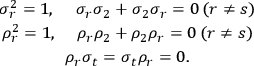
The principle of superposition turned out to be a key component of Hō’s fame in Japan. In 1922, in seeking to apply this principle to the problem of power lines, he rediscovered what is now known as Thévenin’s equivalent circuit theorem, a cornerstone of circuit theory, which every electrical engineering student learns today. The theorem makes the calculations of complicated electrical circuits much easier than they would be if one applied Kirchhoff’s laws directly. Thévenin’s theorem resembles what Edwin Layton called “engineering sciences” (Layton 1971, 567). While the value of this theorem mostly lies in its practicality, it is a mid-level theorem, derived rigorously through theoretical considerations from fundamental principles, namely the principle of superposition and Kirchhoff’s laws. This theorem had been derived previously and sometimes independently by several scientists and engineers, including Hermann von Helmholtz, Léon Charles Thévenin, Hans Ferdinand Mayer and Edward Lawry Norton. Although presented in different formulations, the theorem is essentially a way to substitute a part of a complex circuit with a simpler equivalent circuit consisting of a certain voltage source and a resistance. Thévenin formulated the theorem as follows:
Assuming any system of linear conductors connected in such a manner that to the extremities of each one of them there is connected at least one other, a system having some electromotive forces,,
,
,
, no matter how distributed, we consider two points
and
belonging to the system and having actually the potentials
and
. If the points
and
are connected by a wire
, which has a resistance
, with no electromotive forces, the potentials of points
and
assume different values of
and
, but the current
flowing through this wire is given by the equation
, in which
represents the resistance of the original system, this resistance being measured between the points
and
, which are considered to be electrodes. (Suchet 1949, 843–844)
The proof can be stated simply. Here is a textbook presentation of Thévenin’s proof without much change from the original. Let us define the following four configurations:
 and
and
 are not
connected as in fig. (
are not
connected as in fig. (2Configuration I' is defined as the one where
 and
and
 are connected, and
there is a voltage source of
are connected, and
there is a voltage source of
 at point
 . The voltage source is connected in the
opposite direction to
. The voltage source is connected in the
opposite direction to
 and
and
 , so that there is no current between them as in fig. (7.2).
3Configuration II is defined as the system having the same resistance as
Configuration I' but no voltage source, except the one at
 in the opposite direction
to the one in Configuration I' as in fig. (7.3).
in the opposite direction
to the one in Configuration I' as in fig. (7.3).
4Configuration III is the system where
 and
and
 are connected by a wire
of resistance
are connected by a wire
of resistance
 as in fig. (7.4).
Fig. 7.1: Configuration I: Unconnected circuit.
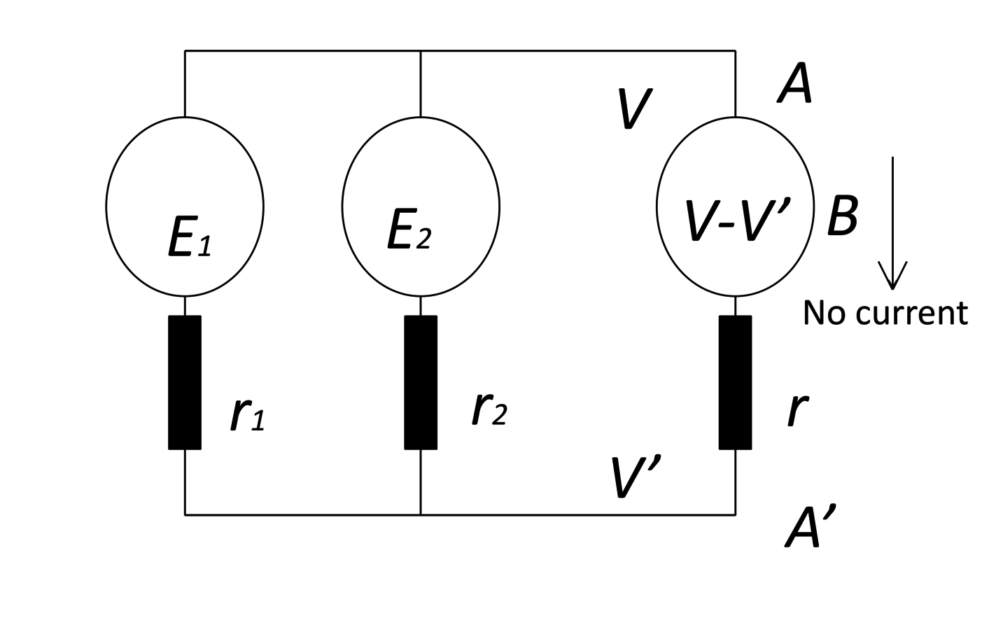
Fig. 7.2: Configuration I': Circuit with an added voltage source.
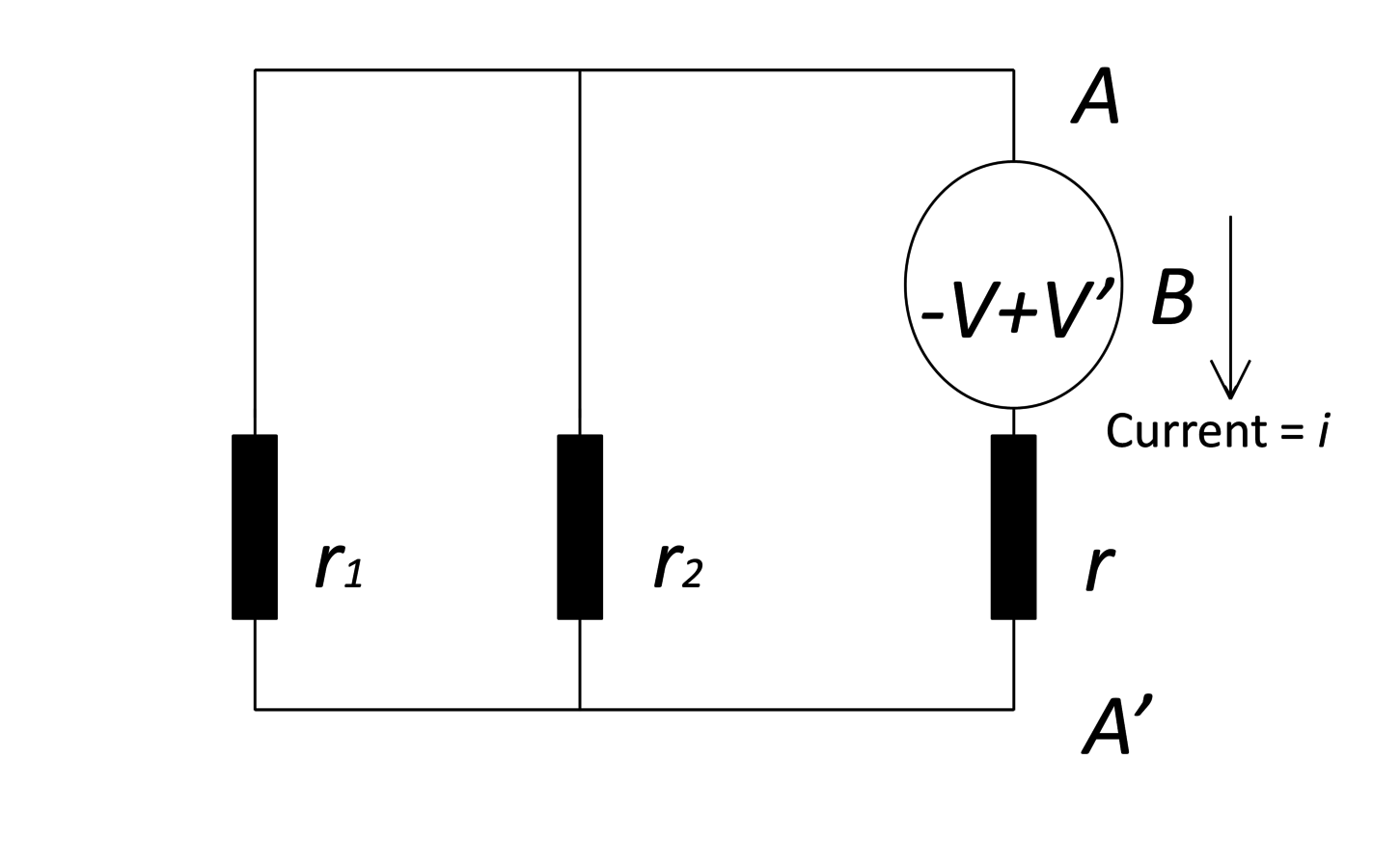
Fig. 7.3: Configuration II: Thévenin’s equivalent circuit.
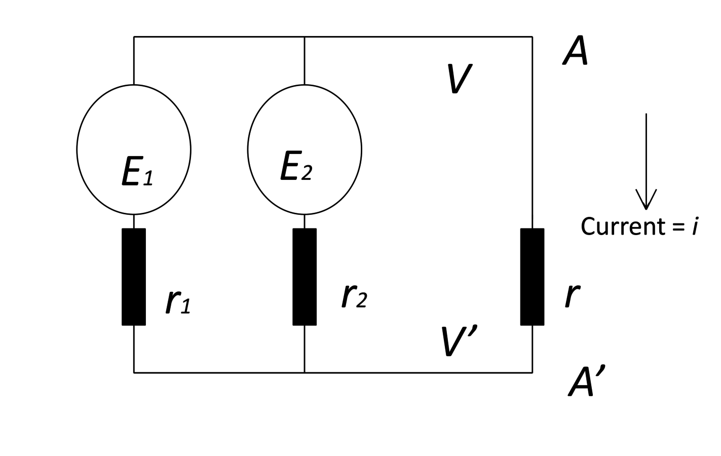
Fig. 7.4: Configuration III: Connected circuit.
Since there is no current between
 and
and
 in Configuration I',
Configuration I' gives the same voltages and currents at each point as in
Configuration I. According to the principle of superposition, Configuration III can
be obtained by adding Configuration I' to Configuration II. Since there is no
current at
in Configuration I',
Configuration I' gives the same voltages and currents at each point as in
Configuration I. According to the principle of superposition, Configuration III can
be obtained by adding Configuration I' to Configuration II. Since there is no
current at
 , the current at
 in Configuration III comes only from Configuration
II, which is what the theorem states.
in Configuration III comes only from Configuration
II, which is what the theorem states.
Hō reached a form of this theorem without knowing that others had
already found it. In his 1922 paper on power transmission, Hō devised a way to
calculate the effects of an accidental grounding of a transmission line, by
ingeniously using the principle of superposition. The result was the same as Thévenin’s
theorem, except that Hō discussed an alternating current circuit instead of a direct
current circuit and grounding instead of shorting. Hō’s proof was equivalent to
Thévenin’s. Hō considered the transmission line grounded by a wire
with impedance
 as in fig. (7.5). Suppose the voltage at point
 is given by:
|
7.4 |
where
 ,
,
 ,
,
 are the amplitude, angular frequency, and initial phase of the voltage.
There will be no current through
are the amplitude, angular frequency, and initial phase of the voltage.
There will be no current through
 if there is an electromotive force with the
same strength but in the opposite direction as in fig. (7.6). If there is an
electromotive force with the same strength but in the opposite direction at the
same point as in fig. (7.7), then those two electromotive forces cancel each other
and the result should be the same as fig. (7.5). Since fig. (7.7) can be obtained by
superposing fig. (7.6) and fig. (7.8), the current through
if there is an electromotive force with the
same strength but in the opposite direction as in fig. (7.6). If there is an
electromotive force with the same strength but in the opposite direction at the
same point as in fig. (7.7), then those two electromotive forces cancel each other
and the result should be the same as fig. (7.5). Since fig. (7.7) can be obtained by
superposing fig. (7.6) and fig. (7.8), the current through
 can be calculated by fig. (7.8) (Hō 1922).
Although this was a special case of what we today call Thévenin’s theorem, Hō’s proof was the same as the proof for the general case. Because of this work, the theorem is called the Hō-Thévenin theorem in Japan, with Hō’s name firmly attached. Whether Hō is entitled to be named one of the discoverers of this theorem is not the issue here. What is of interest is that the principle of superposition was so central to Hō’s work.
Nishina was situated deeply in this tradition of alternating current theory, in which the principle of superposition dominated. Not only did Nishina read Hō’s textbooks and attend his classes, he wrote his bachelor’s thesis along the line manifested by Hō’s derivation of the Hō-Thévenin theorem. The main question in Nishina’s thesis was how unbalanced loads would affect an alternator, a motor, or a rotary transformer in a polyphase system. It relied heavily on Hō’s and Steinmetz’s work (Nishina 1918).
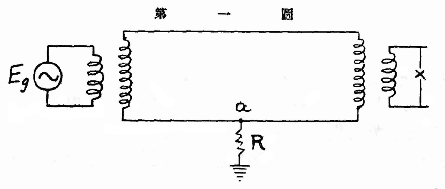
Fig. 7.5: Grounded circuit (Source: Hō 1922, 193).
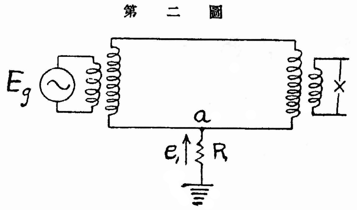
Fig. 7.6: Circuit equivalent to non-grounded circuit (Source: Hō 1922, 194).
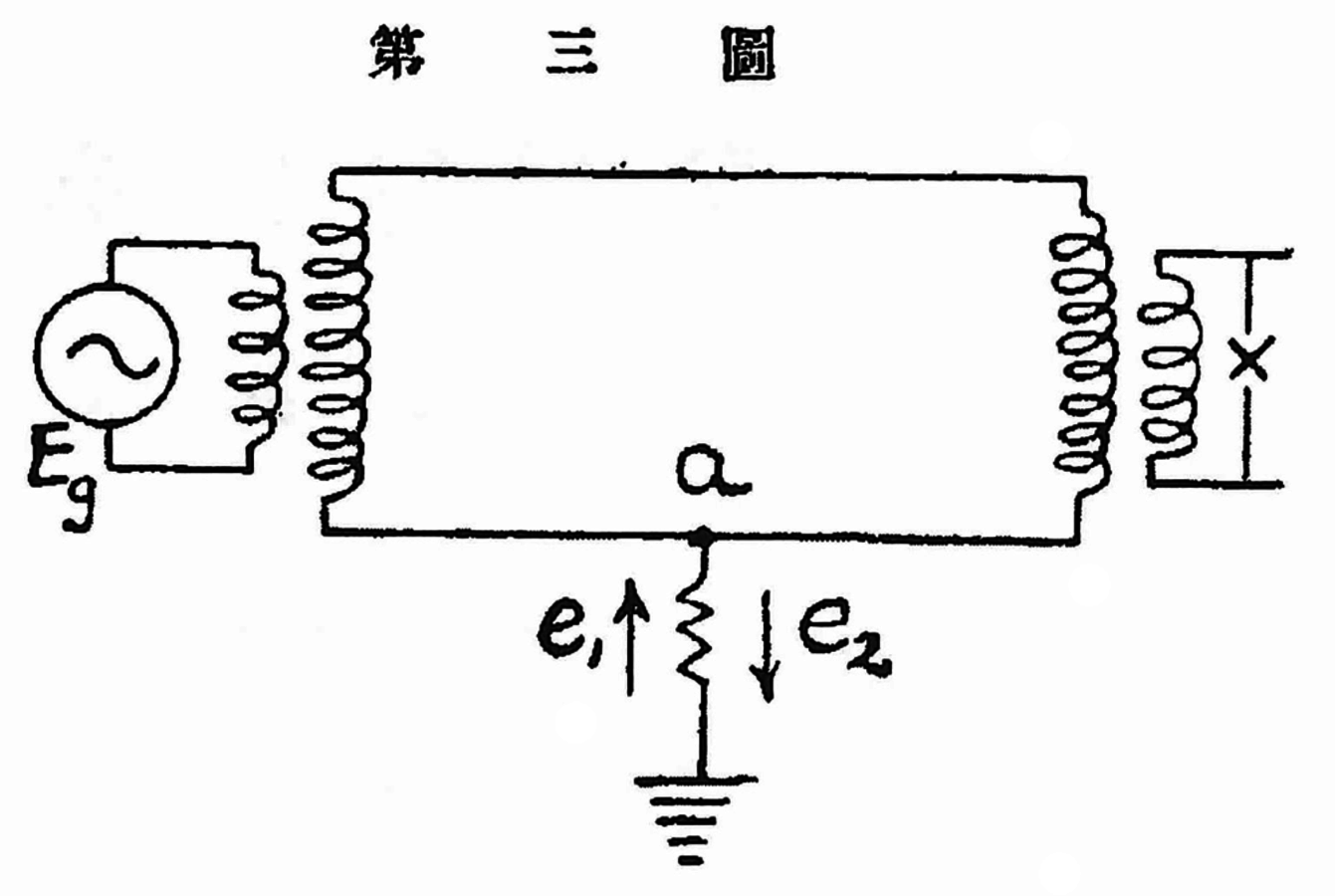
Fig. 7.7: Circuit equivalent to grounded circuit (Source: Hō 1922, 194).
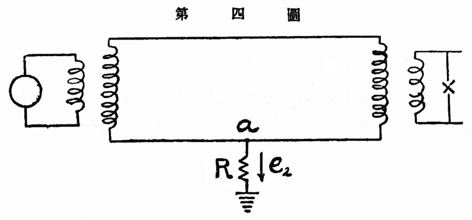
Fig. 7.8: Hō’s equivalent circuit (Source: Hō 1922, 194).
Nishina started his bachelor’s thesis with definitions of a few main concepts. In an
 -phase
system, if the voltage is equal in all branches and the phase difference between the branches is one
-phase
system, if the voltage is equal in all branches and the phase difference between the branches is one
 th, the system is called symmetrical. If not, it is asymmetrical. If
the sum of the power in all
th, the system is called symmetrical. If not, it is asymmetrical. If
the sum of the power in all
 branches is constant, it is called balanced, if not,
unbalanced. A symmetrical system, for example, can be unbalanced when loaded
unequally.
branches is constant, it is called balanced, if not,
unbalanced. A symmetrical system, for example, can be unbalanced when loaded
unequally.
According to Nishina, the problem of imbalances in three-phase systems was very practical. Nishina thought that, as the centralization of the electrical power supply continued, the three-phase system would be the most efficient for generating and transmitting electric power. However, after the introduction of the single-phase commutator motor, there arose a demand for single-phase electrical power supplies. If a single-phase load was supplied with electricity directly from a three-phase system, the voltage would become unbalanced. Hence, the problem of an unbalanced load would ensue. With such motivating factors in mind, Nishina proceeded to the main part of his thesis, which discussed how unbalanced loads would affect a few types of alternating current device, such as an alternator, a motor and a rotary transformer.
In the case of the alternator, Nishina examined what would happen when loads were connected in an unbalanced fashion to a three-phase alternator (that is when loads were connected to only one or two of the three phases). Treating the problem theoretically, Nishina argued that unfavorable effects would result. Terminal voltage would become “unsymmetrical” both in phase and in magnitude (Nishina 1918, 94–95). This would increase both iron and copper loss, reducing efficiency and producing more heat. The unbalanced load would also cause odd higher harmonics, which would result in an “uncomfortable” humming noise.
In analyzing the unbalanced system, Nishina applied reasoning similar to Hō’s “principle of superposition.” In his discussion of the unbalanced three-phase system, he claimed that it could be considered a superposition of two balanced three-phase systems rotating in opposite directions, or in his words: “An unbalanced polyphase system can be resolved into two balanced components with opposite phase rotations, one positive and the other negative.” Nishina cited R. E. Gilman and Charles LeGeyt Fortescue, who originally “discovered” and “proved” this theorem (Nishina 1918, 20). In his thesis, Nishina reproduced their proof.
The proof goes as follows. Define
 as:
as:
|
7.5 |
where
 is the imaginary unit and
 is the number of the phase.
 ,
,
 ,
,
 ,
,
 , and
, and
 ,
,
 ,
,
 ,
,
 , are terminal voltages of two symmetrical
 -phase systems,
rotating in opposite directions. Since a factor of
-phase systems,
rotating in opposite directions. Since a factor of
 rotates the phase of a
complex number by
rotates the phase of a
complex number by
 , these terminal voltages of the symmetrical
 -phase systems can be written as:
 and
and
 .
Nishina’s claim above states that for any
.
Nishina’s claim above states that for any
 phase system, of which the terminal voltages are
 , there are
 , that satisfy
 Nishina’s proof goes as follows. If the equations above are multipled by
 , then:
|
7.6 |
By summing both sides of the equations, and using the definition of
 , the result is:

|
7.7 |
This determines
 .
.
 can be derived similarly. This derivation indicates Nishina’s familiarity with the idea of analyzing the physical system by separating it into superposed components, as well as with the ways of exploiting the linearity of alternating current circuits, just as Hō had done.
The most interesting aspect of this proof is, however, that it was wrong. Eq. (7.7) is a necessary condition for the original equations for
 and
and
 , but it is not guaranteed that the derived forms of
 and
and
 and the other terminal voltages satisfy the original equations. In fact, they do not
satisfy these equations in general, which one can confirm by simple substitution.
As famously shown by Fortescue (1918), decomposing an
and the other terminal voltages satisfy the original equations. In fact, they do not
satisfy these equations in general, which one can confirm by simple substitution.
As famously shown by Fortescue (1918), decomposing an
 -phase unbalanced system requires
 -balanced components. However, since the actual problems Nishina dealt with were three-phase systems, this theoretical mistake was not catastrophic. In short, Nishina’s thesis arguments were mathematically inaccurate but, probably helped by his physical intuition,15 his conclusions were physically correct.
Nishina’s thesis shows his commitment to Hō’s theoretical tradition of electrical engineering, his close ties to Steinmetz’s tradition,16 and his ability in theoretical and physical reasoning. Nishina’s work was theoretical in the sense that he derived fairly general characteristics of the three-phase system. Although the thesis reveals Nishina’s relative mathematical weakness compared to some of the mathematical wizards entering physics at the time, it nonetheless demonstrates Nishina’s ability to draw physically correct conclusions and highlights his immersion in the Hō tradition, especially his familiarity with Hō’s strategy for exploiting linearity and superposition to represent physical phenomena.
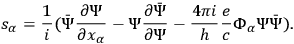
7.3 The Klein-Nishina Formula
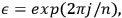
The principle of superposition occupies a central place in quantum mechanics. In particular, the idea plays a crucial role in Dirac’s formulation of quantum mechanics, as manifested by Dirac’s textbook first published in 1930 (Dirac 1930). This book was soon translated into Japanese by Nishina and his students, including Tomonaga Sin-Itiro (Dirac 1936). Hence, it is reasonable to suppose that Nishina’s familiarity with the principle of superposition through electrical engineering was useful to him when learning quantum mechanics and when carrying out quantum theoretical research.
This section and the next closely examine Nishina’s earliest and most important work in theoretical physics, performed in collaboration with Klein, and resulting in the so-called Klein-Nishina formula (Klein and Nishina 1929). I explore how Nishina, along with Klein, actually employed the idea of superposition in his theoretical research in quantum mechanics.
Historically, the Klein-Nishina formula was one of the earliest applications of Dirac’s theory. It was very quickly confirmed experimentally giving strong empirical evidence to support Dirac’s theory, which had various conceptual problems, including the issue of negative energies. Klein and Nishina derived this formula through a semi-classical treatment of Compton scattering. Following Walter Gordon and Dirac, they used Dirac’s relativistic theory of the electron instead of the non-relativistic theory. Such a semi-classical approach for the Compton effect was first explored by Gordon (1926). In his 1926 paper,
Gordon proceeded by comparing classical and quantum mechanical calculations.
He had a relatively simple picture behind his calculation. Incoming radiation
disturbs and imparts motion to an electron through electromagnetic interaction. Gordon first calculated how the incoming radiation would interact with
the electron, both in classical mechanics and quantum mechanics. When moving,
the electron, a charged particle, emits radiation, which Gordon calculated using a
classical electromagnetic formula. He assumed the emitted radiation to correspond to the outgoing X-ray observed
in the experiment.
What Gordon did can be written mathematically as follows. He
assumed that the incoming radiation was a monochromatic plane wave, setting its
(four-)vector potential
 as:
as:
|
7.8 |
where
 is the speed of light,
 the vector that gives the direction of the radiation,
 the frequency of the wave,
 the amplitude of the wave, and
 the index of a four-vector taking the values 1 through 4 (alternatively 0 through 3), whereas
 is the index of a three-vector, taking the values 1 through 3. The first task was
to solve the equation of motion for the electron. For
the quantum mechanical treatment of this problem, Gordon chose to use the Klein-Gordon
equation:
is the index of a three-vector, taking the values 1 through 3. The first task was
to solve the equation of motion for the electron. For
the quantum mechanical treatment of this problem, Gordon chose to use the Klein-Gordon
equation:
|
7.9 |
where
 is the wave function. In the presence of the above-mentioned incoming radiation,
this equation can be solved to first order, giving:
is the wave function. In the presence of the above-mentioned incoming radiation,
this equation can be solved to first order, giving:
|
7.10 |
where
 ,
,
 , and
, and
 are all inner products
of four vectors.
are all inner products
of four vectors.
In classical mechanics, where the electron can be considered a point mass, the electromagnetic wave resulting from its motion is easily calculated. In particular, the frequency of this wave is trivially the same as the frequency of the moving electron. The quantum mechanical treatment required a more complicated procedure, since the electron needed to be considered not as a point mass but as a spatially distributed wave.
From the specific solutions of the equation, Gordon wrote up the general form of the solution as an arbitrary superposition of them:
|
7.11 |
where
 is a weight and
 is a normalization factor (Gordon 1926, 125). Gordon assumed that the electric current in quantum
mechanics should take the following form:
is a normalization factor (Gordon 1926, 125). Gordon assumed that the electric current in quantum
mechanics should take the following form:
|
7.12 |
Then he plugged this expression into the classical electromagnetic formula for the retarded potential,
|
7.13 |
which gives the electromagnetic field caused by the current. Here,
 is the spatial
distance between the volume element
is the spatial
distance between the volume element
 of the integral and the point in question. The brackets
 indicate that
 in
in
 should be substituted by
 . Then,
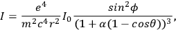
Gordon calculated the frequency and intensity of the induced radiation. The
result, according to Gordon, agreed with the one obtained by Dirac in his 1926 paper:
. Then,
Gordon calculated the frequency and intensity of the induced radiation. The
result, according to Gordon, agreed with the one obtained by Dirac in his 1926 paper:
|
7.14 |
where
 is the angle between the electric field and the observed direction,
 the angle
between the direction of the incoming radiation and the observed direction,
the angle
between the direction of the incoming radiation and the observed direction,
 the intensity of the incoming radiation, and
 the distance between the point of
scattering and the point of observation. It was approximately identical to the
formula obtained by Arthur Compton.
the distance between the point of
scattering and the point of observation. It was approximately identical to the
formula obtained by Arthur Compton.
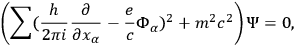
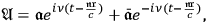
Klein and Nishina adopted Gordon’s approach, but used Dirac’s relativistic theory of electrons instead of the Klein-Gordon equation and the formula for the electron current given by Gordon. The first step is to solve the Dirac equation for a free electron, whose spin is zero on average, and for an electron in a monochromatic unpolarized radiation. The Klein-Gordon equation is replaced by the Dirac equation:
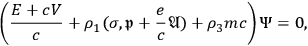
|
7.15 |
in which
 are (three-)vectors of 4 by 4 matrices given by Dirac, whose elements satisfy the following relations:
|
7.16 |
Suppose the monochromatic radiation is given by a vector potential of the following form:
|
7.17 |
where
 is the unit vector in the direction of the incoming wave. Nishina and Klein calculated the solution up to first order:
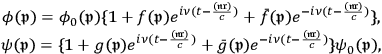
|
7.18 |
in which
 and
and
 are eigenfunctions of a free electron:

|
7.19 |
and
 and
and
 are constant matrices, determined by:
|
7.20 |
Here,
 and
and
 or
or
 and
and
 respectively depend on the electric and magnetic fields of the radiation,
 and
and
 :
:
|
7.21 |
The general solution of the wave equations arises from a superposition of all possible solutions of the form (7.18) up to the considered approximation.
|
7.22 |
The second step is to calculate the current density using this solution. The following formula for the current density is given by Dirac in his 1928 paper (Dirac 1928):
|
7.23 |
Inserting the solutions above, we have:
|
7.24 |
Using the formula for the retarded potential, this electric current causes radiation
 :
:
|
7.25 |
where
 means the integration
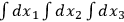 over the entire region available to the electron.
By further calculation, and using Maxwell’s equations and various relations that the Dirac matrices satisfy, we have for the magnetic field
 :
:
|
7.26 |
Here,
 is a unit vector in the direction of observation,
 is the frequency of the outgoing radiation, and the following abbreviations are used:
|
7.27 |
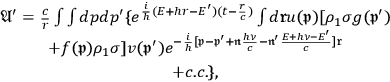
The fourth and final step is to calculate an observable physical quantity, such as the intensity of scattered radiation. For this, we need to calculate the expectation value of
 . Beside obviously meaning a long calculation, including manipulations of Dirac matrices, this also involves the question of how to evaluate expectation values, which I discuss closely in the following section. The result is:
|
7.28 |
From this, if we write the angle between the observation direction and the direction of the incoming wave as
 , and the angle between the observation direction and the electric force of the incoming wave as
 , the intensity of the outgoing radiation is:

|
7.29 |
where
 ,
,
 is the intensity of the incoming radiation.
One could point out that this particular approach to this problem is reminiscent of electrical engineering in various ways. After all, calculating electromagnetic waves emitted by electric current is one of the foremost topics of electrical engineering.
7.4 Superposition of States in the Klein-Nishina Paper
Although the fourth step above might appear to be a very lengthy and complex, but straightforward calculation, in reality, it was more than that. Yazaki Yūji (1992) has clarified Klein and Nishina’s thought process by closely studying the Klein-Nishina paper and the extensive archival materials that Nishina left at RIKEN. According to Yazaki, the main physical problem Nishina and Klein faced was to determine the initial and final states of the electron and to calculate the
average of the magnetic field. The procedure for calculating an average of a physical quantity was neither standardized nor clear at this point. It was even less apparent because of the semi-classical approach. Today, we know that we need to calculate contributions from orthogonal states, but in their time, the notion of orthogonality and its relevance to the calculation of a quantum statistical average was not clear. Klein and Nishina thought that they would take the average of two “independent states,” such as the two states having magnetic moments (spin) in opposite directions. However, the states for spin up and down along the
 -axis satisfy the Dirac equation only when
 Eventually, they solved this problem using the method of Lorentz transformation that Klein developed (see below on page
My aim here, however, is not to revisit their physical considerations, which Yazaki has already studied. Instead I intend to make explicit and confirm that the idea of superposition of states did indeed play an important role in the calculation of expectation values Klein and Nishina carried out.
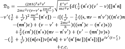
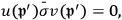
Since
 is a sum of bilinear terms such as
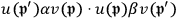 , where
 and
and
 are certain matrices, Klein and Nishina had to calculate these terms. The authors reduced all the terms to the calculation of
 and
and
 . For these terms, Klein and Nishina derived the following values:
|
7.30 |

|
7.31 |
where the overbar means average.
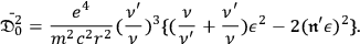
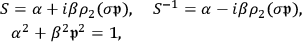
The factor of 2 in this equation is remarkable, especially because eq. 20 in the Klein-Nishina paper (Klein and Nishina 1929, 858) states:
|
7.32 |
How did they reach these values? This part of their calculation hinged on their choice for the initial and final states of the electron.
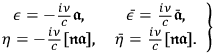
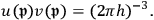
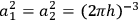
For the initial state, it seems appropriate to choose spin up and down states as two independent states. To explain this choice, it is necessary to explicitly fix spinor and matrix elements. Klein and Nishina chose
 and
and
 to be diagonal. Hence:
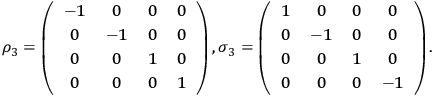
|
7.33 |
From the Dirac equation for free electrons, it follows that in the case of
 ,
,

|
7.34 |
Thus, one can choose two independent solutions, with either
 ,
,
 or
or
 ,
,
 being nonzero. Hence, the solutions are:
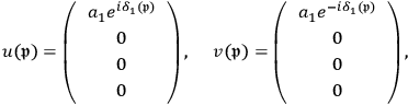
|
7.35 |
and
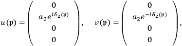
|
7.36 |
where
 , and
, and
 are phases that can be chosen freely.
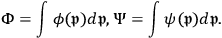
For the final state, since the electron is not at rest, the equations are not so simple. As Yazaki (1992) shows, they solved this by introducing a contact transformation:
|
7.37 |
where,
 are given by the following equations:
|
7.38 |
They define
 and
and
 by:
by:

|
7.39 |
Then the Dirac equations take the same form as for
 :
:

|
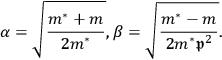
7.40 |
In the case of the final state of the Compton effect, Klein and Nishina claim both
 and
and
 must be considered finite (Klein and Nishina 1929, 864). Hence, it appears the wave functions for the final state have both components, namely:
|
7.41 |
In other words, for the final state of the electron, they combined (or superposed) the two independent solutions
 with variable phase factors. Thus, behind the scenes, Nishina, with Klein, went back to his old friend from his electrical engineering student years—the principle of superposition—to carry out his first and most important work in quantum mechanics.
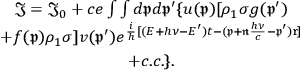
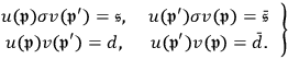
For the value of
 , Klein and Nishina employed physical considerations and direct calculation. They claim the final state “should contain the two independent solutions with equal strength,” the average of
 over phases must vanish (Klein and Nishina 1929, 866). Hence the expectation value of
 , the magnetic moment of the electron, is zero. The same value can be derived through straightforward calculation by plugging in the expression in eq. (7.41), and averaging over
 and
and
 . As for
 , one can get
 by inserting the expression in eq. (7.41).
Klein and Nishina did not clearly show how they justified this procedure for calculating a statistical average. This procedure of summing over phases did not appear in the previous theory of the Compton effect, such as Gordon’s (1926). Although Klein and Nishina did not state it explicitly, they probably took into consideration that different phases give different directions of spin, not unlike Steinmetz’s alternating current theory, where different imaginary numbers give different directions of vectors in vector diagrams. Summation over phases meant summation over the direction of the magnetic moment. At least for the initial state, the physical meaning was then clear. As for the final state, the situation was somewhat different, because the physical meanings of
 and
and
 were not transparent. They probably justified their assumptions by showing that
 vanishes by direct calculation.
Since they were considering unpolarized light as the incoming radiation, the average of the magnetic moment in the final state should also be zero.
vanishes by direct calculation.
Since they were considering unpolarized light as the incoming radiation, the average of the magnetic moment in the final state should also be zero.
Since summation over phases eliminates non-diagonal elements and sums diagonal elements, this procedure can be considered equivalent to taking a trace. Because the density matrix in this case is proportional to the unit matrix, this procedure agrees with a quantum statistical calculation for a mixed state. A mathematical theory about this procedure of quantum statistics had already been presented by John von Neumann in 1927, see (von Neumann 1927). Klein and Nishina were likely unaware of the relevance of Neumann’s paper but managed to do a mathematically-equivalent calculation relying on physical considerations (if they had noticed it, their calculation would have been much different; taking a trace from the beginning would have made the calculation much shorter and easier).
7.5 Conclusion
As I wrote at the beginning of this paper, I am not claiming any deterministic, causal connections. It would be ridiculous to claim that Nishina worked on quantum mechanics because he studied electrical engineering. Nor do I claim that Nishina took a certain research style in quantum mechanics different from others because of his electrical engineering background. What I claim is that quantum mechanics, not only its experiments but also its theoretical research, might not be as disconnected from other fields of investigation, such as engineering, as we might assume. In terms of theoretical practices, there are some similarities between alternating current theory and quantum physics, at least in the way they were experienced by a person like Nishina.
Therefore, the fact that Nishina was originally trained in electrical engineering does not mean that Nishina started learning quantum mechanics “from scratch.” Nishina’s engineering training probably prepared him for theoretical research in quantum mechanics to some extent. At least in this limited sense, it seems the institutional and pedagogical developments in engineering helped introduce theoretical research in quantum mechanics into Japan.
Acknowledgements
This work is partially supported by the Ministry of Education, Culture, Sports, Science and Technology (MEXT) Grant-in-Aid for Scientific Research C (Kakenhi) # 21500976.
References
Aichi, Keiichi (1923). Denshi no jijoden: Tsūzoku kagaku kōgi (The autobiography of an electron: A popular science account). Tokyo: Shōkabō.
Bartholomew, James R. (1989). The Formation of Science in Japan: Building a Research Tradition. New HavenLondon: Yale University Press.
Brown, Laurie M. (2002). The Compton Effect as One Path to QED. Studies in History and Philosophy of Modern Physics 33: 211-249
Dalitz, Richard H. (1990). Another Side to Paul Dirac. In: Reminiscences about a Great Physicist: Paul Adrien Maurice Dirac Ed. by Behram N. Kursunoglu, Eugene P. Wigner. Cambridge: Cambridge University Press 69-92
Dirac, Paul A. M. (1926). Relativistic Quantum Mechanics with an Application to Compton Scattering. Proceedings of the Royal Society A 111: 405-423
- (1928). The Quantum Theory of the Electron. Proceedings of the Royal Society A 117: 610-624
- (1930). The Principles of Quantum Mechanics. Oxford: The Clarendon Press.
- (1936). Ryōshi rikigaku (Quantum mechanics). Tokyo: Iwanami Shoten.
Fortescue, Charles L. (1918). Method of Symmetrical Co-ordinates Applied to the Solution of Polyphase Networks. AIEE Transactions 37, part II: 1027-1140
Galison, Peter L. (1997). Image and Logic: A Material Culture of Microphysics. Chicago: The University of Chicago Press.
- (2000). The Supressed Drawing: Paul Dirac's Hidden Geometry. Representation 72: 145-166
- (2003). Einstein's Clocks, Poincaré's Maps: Empires of Time. New York: W. W. Norton & Company.
Gibson, Charles R. (1911). The Autobiography of an Electron: Wherein the Scientific Ideas of the Present Time Are Explained in an Interesting and Novel Fashion. Philadelphia, London: J.B. Lippincott Company, Seeley & Co., Limited.
Gordon, Walter (1926). Der Comptoneffekt nach der Schrödingerschen Theorie. Zeitschrift für Physik 40: 117-133
Hirosige, Tetu (1973). Kagaku no shakaishi: Kindai Nihon no kagaku taisei (Social history of science: Scientific regime in modern Japan). Tokyo: Chūō Kōron Sha.
Hō, Hidetarō (1912). Kōryū riron (Alternating current theory). Tokyo: Maruzen Kabushiki Kaisha.
- (1922). Sōdensen no secchi to chōjō no ri (Grounding of power line and the principle of superposition). Denki Gakkai zasshi (Journal of the Institute of Electrical Engineers of Japan) 42: 193-198
- (1923). Hadō shindō oyobi hirai (Wave, vibration, and arrestoring). Tokyo: Maruzen.
Ito, Kenji (2002) Making Sense of Ryōshiron (Quantum Theory): Introduction of Quantum Physics into Japan, 1920–1940. phdthesis. Harvard University
Kim, Dong-Won (2007). Yoshio Nishina: Father of Modern Physics in Japan. New YorkLondon: Taylor & Francis.
Klein, Oskar, Yoshio Nishina (1929). Über die Streuung von Strahlung durch freie Elektronen nach der neuen relativistischen Quantendynamik von Dirac. Zeitschrift für Physik 52: 853-868
Kline, Ronald R. (1992). Steinmetz: Engineer and Socialist. Baltimore: Johns Hopkins University Press.
Kragh, Helge (1990). Dirac: A Scientific Biography. Cambridge: Cambridge University Press.
Layton, Edwin (1971). Mirror Image Twins: The Communities of Science and Technology in Nineteenth Century America. Technology and Culture 12: 562-580
Mizuno, Toshinojō (1912). Denshiron (The electron theory). Tokyo: Maruzen Kabushiki Kaisha.
- (1918). Densi no katsudō (Activities of the electron). Tokyo: Maruzen Kabushiki Kaisha.
Nagaoka, Hantarō (1912). Genkon no denkigaku (Studies of electricity today). Tokyo: Kōdōkan.
von Neumann, John (1927). Wahrscheinlichkeitstheoretischer Aufbau der Quantenmechanik. Nachrichten von der Gesellschaft der Wissenschaften zu Göttingen 1: 245-272
Nishina, Akira (1975). Memories of Dr. Nishina Yoshio. Takahashigawa 32: 4-19
Nishina, Yoshio (1918). Effects of Unbalanced Single-Phase Loads on Poly-Phase Machinery and Phase Balancing (B. A. Thesis)..
- (1946). Watashi wa nani o yondaka (What I have read). In: Genshiryoku to watashi: Nishina Yoshio hakase ikōshū (Atomic power and I: Posthumous collection of Dr. Nishina Yoshio's writings) Tokyo: Gakufū Shoten 224-230
Pyenson, Lewis (1982). Audacious Enterprise: The Einsteins and Electrotechnology in Late Nineteenth-Century Munich. Historical Studies in the Physical Sciences 12: 373-392
- (1985). The Young Einstein: The Advent of Relativity. Bristol: Hilger.
Steinmetz, Charles Proteus (1893). Complex Quantities and Their Use in Electrical Engineering. Proceedings of the International Electrical Congress
Stuewer, Roger H. (1975). The Compton Effect: Turning Point in Physics. New York: Science History Publications.
Suchet, Charles (1949). Léon Charles Thévenin (1957–1926). Electrical Engineering 68: 843-844
Sugiura, Yoshikatsu (1927). Über die Eigenschaften des Wasserstoffmoleküls im Grundzustande. Zeitschrift für Physik 45: 484-494
Yagi, Eri (1974). Hantaro NAGAOKA. In: Dictionary of Scientific Biography New York: Charles Scribner's Sons 606-607
Yazaki, Y. (1992). Klein-Nishina kōshiki dōshutsu no katei: Riken no Nishina shiryō o chūshin ni (How was the Klein-Nishina formula derived?: Based mainly on the source materials of Y. Nishina in RIKEN). Kagakushi Kenkyu
Yukawa, Hideki (1935). On the Interaction of Elementary Particles I.. Proceedings of the Physico-Mathematical Society of Japan 17(3): 48-57
Footnotes
The earliest known book on Newtonian physics in Japan is Shizuki Tadao’s liberal translation in 1798 of John Keill’s Introductiones ad Veram Physicam et Veram Astronomiam (1725).
One example, other than Nishina Yoshio’s work with Oskar Klein described below, is Sugiura Yoshikatsu’s work on the Heitler-London method, see (Sugiura 1927).
Following the common academic convention, I write Japanese names in the traditional order, the family name first, the given name second.
For the history of the Compton effect, see (Stuewer 1975; Brown 2002). For the historical background and significance of the Klein-Nishina formula in relation to Dirac’s relativistic quantum mechanics, see, for example (Kragh 1990).
“Higher School” kōtō gakkō in pre-World War II Japan was a liberal arts institution of higher education, and is not the same as a high school in the United States, for example.
Other important pre-quantum mechanical topics in physics that had practical implications were spectroscopy and X-ray physics, which provided training grounds and institutional bases for experimental atomic physicists. Nishina was familiar with these traditions, but I do not discuss this issue here.
Nishina Akira, a nephew of Yoshio’s, remembered that when Nishina’s elder brother Teisaku mentioned that Yoshio was studying electricity at a party to celebrate Yoshio’s return to Japan in 1929, Teisaku emphasized how Japan was backward as far as the study of electricity was concerned and asked the other guests for support for Yoshio (Nishina 1975).
For a biography of Steinmetz, see (Kline 1992).
Steinmetz’s innovation in alternating current theory was the use of imaginary numbers in understanding alternating current circuits. Steinmetz replaced vector diagrams with imaginary numbers.
In the following discussion, I use the 1923 version of the book (Hō 1923), which probably better represents the instruction that Nishina received in his student years.
The assumption that the coil is infinitely small is equivalent to substituting for the actual curve a flat line within that length, that is equivalent to the first-order approximation.
Nishina could have decomposed an arbitrary unbalanced three-phase system into three, rather than two, symmetrical systems: two rotating in opposite directions and one not rotating at all. Nishina used the reverse component to show the production of higher harmonics and other undesirable effects. These qualitative conclusions did not change significantly whether or not one took the stationary component into consideration.
As for Steinmetz’s tradition, see (Kline 1992).
Yazaki’s articles are unfortunately not in English. For a brief English account of his articles, see (Brown 2002).